Desurveying computes the geometry of a drillhole in three-dimensional space based on its collar location and the raw dip (or inclination), azimuth (or direction) and depth data of one or more surveys. The resulting geometry is a polyline – a connected series of (X, Y, Z) coordinates used to find the composite locations.
Only under ideal conditions will the path of a drilled hole follow the original dip and azimuth established at the top of the hole. It is more usual that it will deflect away from the original direction as a result of layering in the rock, the variation in the hardness of the layers, and the angle of the drill bit relative to these layers. The drill bit will be able to penetrate the softer layers easier than the harder layers, resulting in a preferential direction of drill bit deviation.
Leapfrog implements 3 different algorithms for interpretation of desurveying. Understanding how each works will help you select the correct one for your purpose.
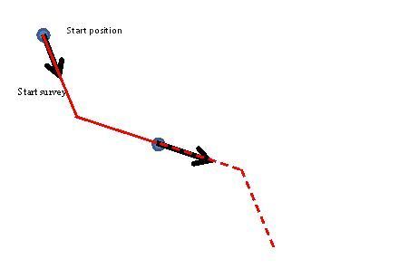
Drillhole desurveying is an important part of model building and can impact significantly on the volume of the calculated geological units. In its simplest form the problem of drillhole desurveying is one of finding the most reasonable path where we know:
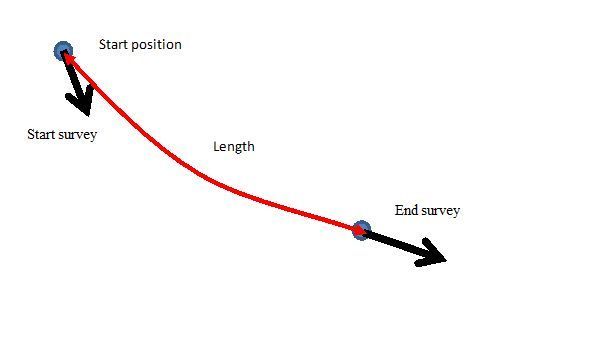
1) the starting survey
2) the starting position
3) the end survey
4) distance between the start and end
The arrangement of this data is shown in Figure 1.
Given the limited information there are a large number of paths the drillhole could take between the survey measurements, but given the physical constraints imposed by a drilling, the smoother paths are more likely.
There are a large variety of algorithms, available with a variety of confusing names. Leapfrog implements 3 different algorithms, which cover the majority of practical circumstances encountered.
1) The basic tangent algorithm
This algorithm (Figure 2) assumes the drillhole maintains the direction given by the last survey measurement until it encounters a new measurement.
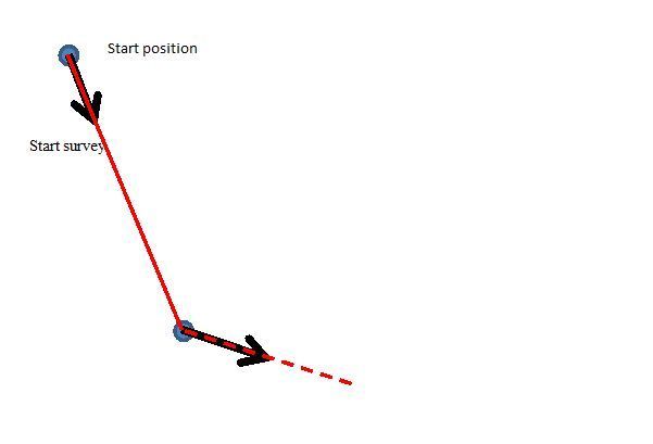
This implies that the drillhole makes sharp jumps in direction whenever a measurement is taken. This seems quite unlikely except when the drillhole is being used to define a trench. In this case Leapfrog allows users to identify the data as a trench on the collar table and this is when the basic tangent algorithm is used.
2) The spherical arc or minimum curvature algorithm
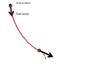
The spherical arc algorithm (Figure 3) is the simplest and best explanation that fits the facts. It matches the survey at the starting and end positions exactly and the curvature is constant between these two measurements. At the survey points the direction remains continuous, so there are no unrealistic sharp changes in direction.
This is the default algorithm in Leapfrog and downhole distances are desurveyed exactly as distances along a circular arc.
3) The balanced tangent algorithm
The balanced tangent algorithm (Figure 4) again uses straight lines, but attempts to improve the accuracy of the tangent algorithm by assigning equal weight to the starting and end survey measurements. It is an improvement on the raw tangent algorithm but still suffers from an unrealistic discontinuity in the drillhole path. That said it is a better approximation to the overall drillhole path and provided the spacing between measurements is small the results are reasonably accurate.
So which is best?
With Leapfrog software we recommend the default is the spherical arc method, because it models the available data in the simplest manner consistent with the facts. Many software packages allow the user to interpolate the survey measurements to reduce the size of straight line segments and create a smoother path. If you use very small segments in the tangent algorithms the results approach the default spherical arc used by Leapfrog. The price is that it takes additional time.
The errors increase with the amount of curvature, so the errors will be small for drillholes that are approximately straight.
So why does Leapfrog provide the balanced tangent algorithm?
Often the user will have wireframes or models that have been created with the tangent methods in other packages. It is not practical to redo much of this work and the need to be consistent is more important than the accuracy of the algorithm.
All desurveying methods only give an interpretation of the real drillhole path. No hole actually follows a precise spherical or spline curve or a set of straight lines. By selecting the desurvey method which gives the best likely approximation of the 3D reality, the user can ensure that any subsequent modelling of a deposit is as accurate as possible.